
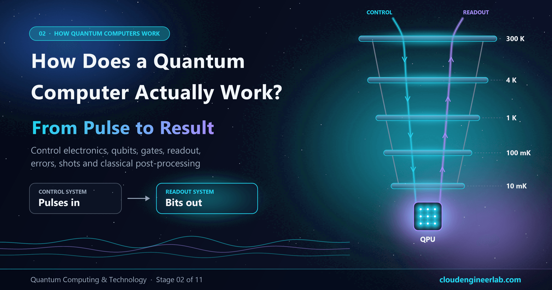
How Does a Quantum Computer Actually Work? From Pulse to Result
Follow one quantum circuit through the real machine: compiler, control electronics, cryostat, qubits, gates, readout, errors, shots and post-processing.
Most explanations of quantum computing stop at the qubit. Superposition, entanglement, a circuit diagram, done. But nobody can run a circuit diagram. Somewhere, a real machine has to turn qc.h(0) into a physical event inside a chip colder than outer space, and turn whatever happens there back into bits on your screen.
That machine is what this post is about. We'll follow a single quantum program from the moment you submit it to the moment you get a result, through every layer it passes: the compiler, the classical control electronics, the refrigerator, the qubits, the gates, the readout system, the errors that creep in, the thousands of repeated shots, and the classical post-processing that turns raw counts into an answer.
This is where quantum computing stops being popular science and becomes engineering. And the first engineering surprise is this: a quantum computer is mostly a classical computer. The quantum part is one small chip. Everything around it, and most of the complexity, is classical.
Stage 02 flagship
This is the flagship post of stage 02, How Quantum Computers Work, in the Quantum Computing & Technology learning path. It assumes the concepts from Superposition, Entanglement and Measurement Explained Without Heavy Mathematics and the machine-level comparison in Classical Computer vs Quantum Computer: What Is Actually Different?. The worked example uses superconducting qubits, the technology behind IBM's and Google's machines, because it has the most layers to explain. Other technologies follow the same architecture with different physics; there's a comparison near the end.
The Architecture: Three Systems Around One Chip
Here is the whole machine on one page:
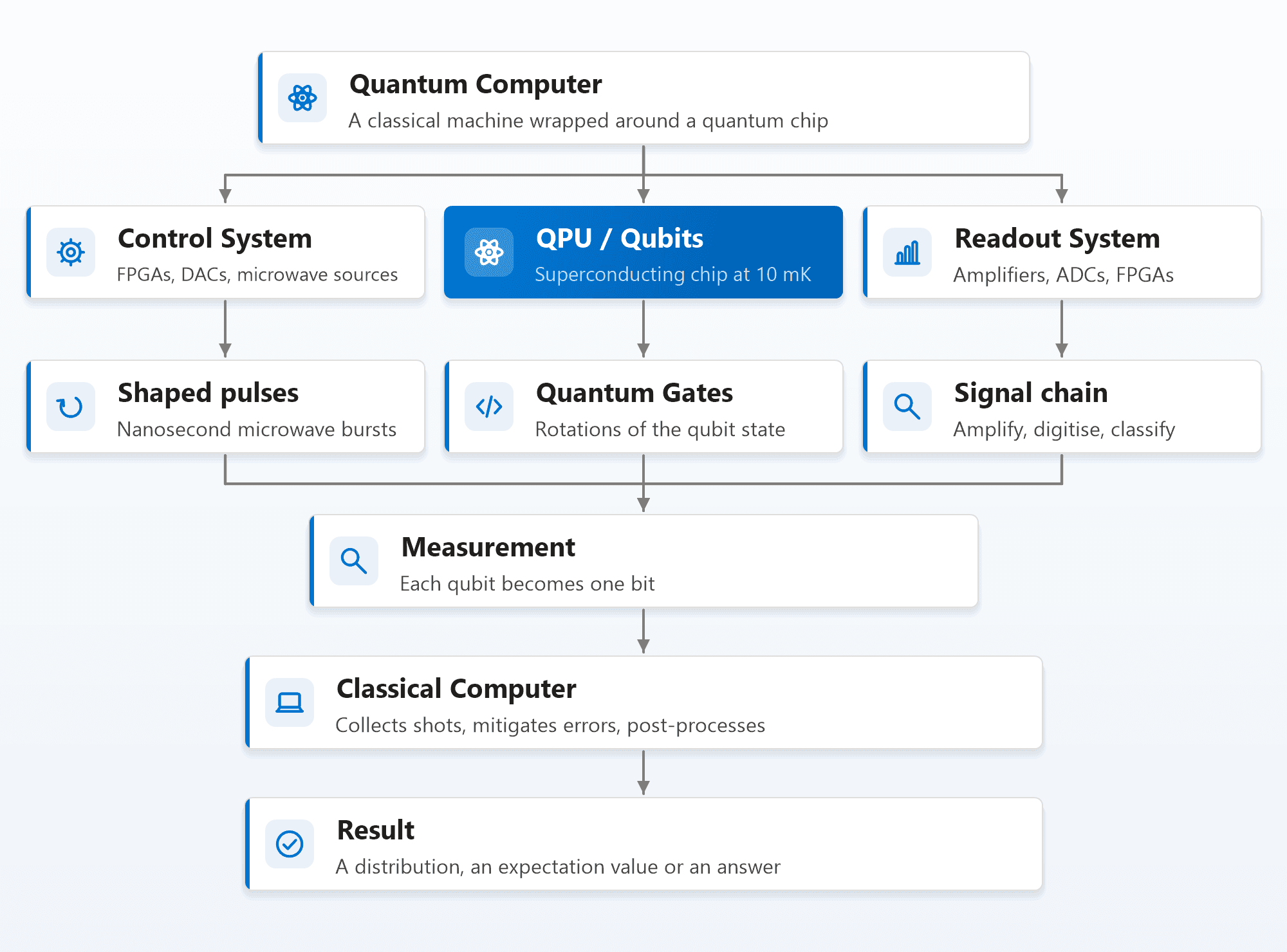
- The control system generates precisely shaped microwave pulses. Each pulse is a quantum gate.
- The QPU is the chip holding the qubits, sitting at the bottom of a dilution refrigerator at about 10 thousandths of a degree above absolute zero.
- The readout system sends a probe signal to each qubit, catches the faint reply, amplifies it, digitises it and decides whether it means 0 or 1.
All three meet at measurement, the moment the quantum state becomes classical bits. From there, a classical computer collects results from thousands of repeated runs, corrects for known errors and computes the final result.
Here's the journey a single job takes through those systems, from your laptop and back:
1. You write and submit a circuit
2. A compiler rewrites it for one specific chip
3. Gates become pulses
4. Control electronics play the pulses
5. The qubits evolve
6. The readout system measures every qubit
7. Reset, and repeat thousands of times
8. Classical post-processing
The rest of this post walks through those steps layer by layer.
Layer 1: The Compiler Turns Your Circuit Into Something a Chip Can Run
The circuit you write is abstract. It assumes any gate can act on any qubit, and that qubits are perfect. Real hardware has neither property. So before anything physical happens, a classical compiler (called the transpiler in Qiskit) rewrites your circuit for one particular QPU. It has four jobs:
- Layout. Choose which physical qubits on the chip play the role of your logical qubits 0, 1, 2 and so on. Good compilers pick the qubits with the best recent error rates.
- Routing. On most superconducting chips, each qubit is physically connected only to a few neighbours. If your circuit needs a two-qubit gate between qubits that aren't connected, the compiler inserts SWAP operations to move quantum states next to each other. Each SWAP costs three two-qubit gates, so routing can multiply a circuit's size.
- Translation. Every QPU supports a small set of native gates. Your H, CNOT and others are rewritten in terms of those. On IBM hardware, for example, a Hadamard becomes a sequence of
rzandsxgates, and a CNOT becomes the chip's native two-qubit gate surrounded by single-qubit rotations. - Optimisation and scheduling. Cancel redundant gates, merge rotations, and decide exactly when each gate starts, packing independent gates in parallel so the circuit finishes as fast as possible.
You can see the effect in a few lines of Qiskit. The circuit you wrote has two gates; the one the hardware runs has more, all from the native set:
from qiskit import QuantumCircuit
from qiskit.transpiler.preset_passmanagers import generate_preset_pass_manager
from qiskit_ibm_runtime import QiskitRuntimeService

backend = QiskitRuntimeService().least_busy(operational=True, simulator=False)

qc = QuantumCircuit(2)
qc.h(0)
qc.cx(0, 1)
qc.measure_all()

pm = generate_preset_pass_manager(backend=backend, optimization_level=1)
isa_circuit = pm.run(qc)              # "ISA" = only gates this chip supports
print(isa_circuit.count_ops())        # e.g. rz, sx and the chip's native 2-qubit gate
Why it matters: every extra gate is another chance for an error. A large share of the practical progress in quantum computing has come from better compilers, not better qubits, because the cheapest error is the gate you never run.
Layer 2: Classical Control Electronics, Where Gates Become Pulses
This is the part most explanations skip, and it's where most of the engineering lives.
A superconducting qubit is controlled with microwaves, the same kind of radio frequency your Wi-Fi uses, at around 4 to 6 GHz. Each qubit has its own frequency, a little different from its neighbours'. To perform a gate, the control system plays a short burst of microwaves at exactly that qubit's frequency.
The pulse's properties map directly onto the gate:
| Pulse property | What it controls | Example |
|---|---|---|
| Frequency | Which qubit responds | Each qubit is tuned to its own frequency, so a pulse at 4.97 GHz affects only the qubit that sits at 4.97 GHz |
| Amplitude × duration | How far the state rotates | Twice the area of an sx pulse gives a full x (NOT) |
| Phase of the microwave | Which axis it rotates around | The same pulse shifted by a quarter cycle rotates around a different axis |
| Shape (envelope) | How cleanly it rotates | Smooth, specially shaped envelopes (such as DRAG pulses) avoid exciting the qubit into unwanted states |
| Start time | When the gate happens | Timed to the nanosecond, so gates on different qubits line up |
A few details reveal how much of a "gate" is really classical engineering:
- Z rotations are usually free. A rotation around the Z axis just shifts the phase reference that every later pulse on that qubit uses. The control system tracks it in software, so a "virtual Z" gate takes zero time and has essentially no error. Compilers exploit this heavily.
- Two-qubit gates need couplers. Two qubits interact through a physical coupling element on the chip. Depending on the design, the control system either drives one qubit at its neighbour's frequency (the cross-resonance approach) or briefly tunes a coupler or qubit frequency with a fast current pulse to switch the interaction on, then off again. These gates take longer and are less accurate than single-qubit gates.
- Everything is calibrated, constantly. The exact frequency, amplitude and shape for each gate on each qubit drift over hours and days as the chip's environment shifts. Automated calibration routines re-measure and re-tune them regularly, and the published "properties" of a cloud QPU (error rates, coherence times) are snapshots from the latest calibration.
Physically, the control system is racks of classical hardware at room temperature:
- FPGAs (programmable logic chips) act as sequencers, playing the right waveform on the right channel at the right nanosecond, and reacting to measurement results in real time.
- DACs (digital-to-analogue converters) and microwave sources turn digital waveforms into real microwave signals, either directly at gigahertz frequencies or by mixing a lower-frequency waveform up to the qubit frequency.
- Separate lines carry DC and fast current pulses for chips with tunable qubits or couplers.
For a chip with 100 qubits, that's several hundred precisely synchronised analogue channels, all feeding a device the size of a fingernail.
| Native operation | How it's physically done | Typical duration (superconducting) |
|---|---|---|
Single-qubit rotation (sx, x) | A shaped microwave pulse at the qubit's frequency | Roughly 20 to 50 nanoseconds |
Z rotation (rz) | A phase change tracked in software | Zero time |
| Two-qubit gate (CZ, ECR and similar) | Microwave drive across a coupler, or a fast flux pulse | Tens to a few hundred nanoseconds |
| Measurement | A microwave probe of the qubit's readout resonator | Roughly 0.5 to 4 microseconds |
| Reset | Wait for the qubit to relax, or measure and flip | Microseconds (active) to hundreds of microseconds (passive) |
Layer 3: The Cryostat, and Why Everything Is So Cold
The QPU lives at the bottom of a dilution refrigerator, the tall, gold-coloured "chandelier" in every photo of a quantum computer. Each plate of the chandelier is a colder temperature stage:
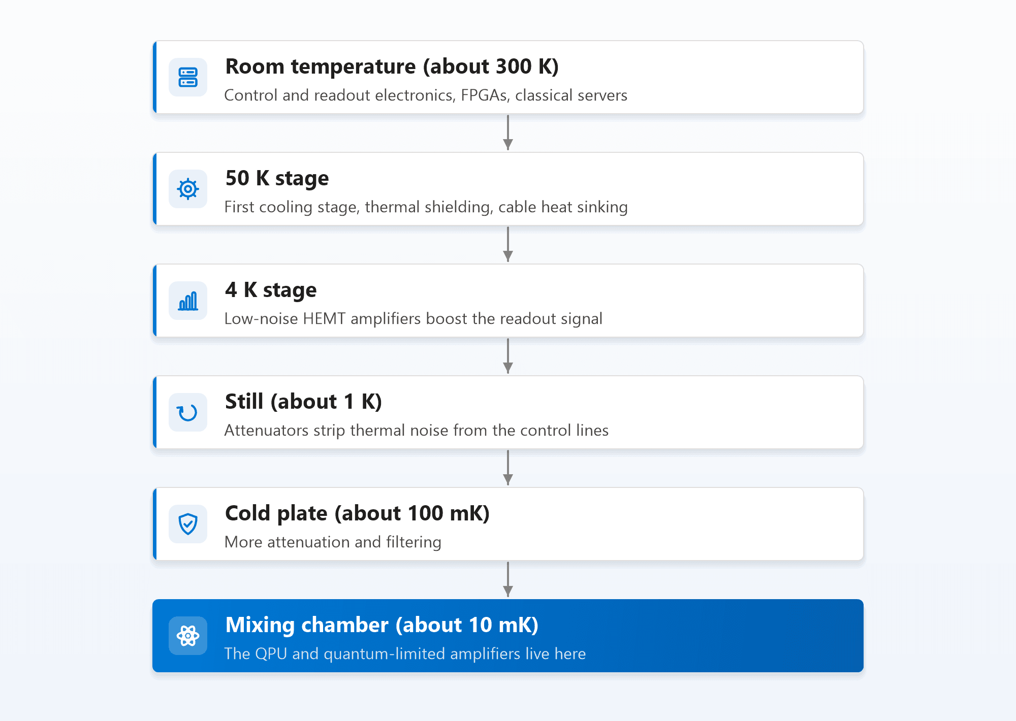
Why so cold? (Why Quantum Computers Need Extremely Cold Temperatures covers this for general readers.) A qubit's two states are separated by a tiny amount of energy, set by its frequency. For a 5 GHz qubit, that energy corresponds to a temperature of about 0.24 kelvin. If the surroundings were warmer than that, random heat would constantly kick the qubit between 0 and 1. At around 10 millikelvin, heat is far too weak to do that, so the qubit reliably sits in 0 until a pulse tells it otherwise. The superconducting metal on the chip also needs to be far below its critical temperature to behave like a perfect, lossless circuit.
Why the attenuators? The control cables carry signals from a 300 K world into a 10 mK one, and a cable carries thermal noise with it. So the input lines pass through a series of attenuators (deliberate signal reducers) and filters on the way down, typically reducing the signal by a factor of about a million in total. The pulses are generated much stronger than needed at room temperature, so that after attenuation they arrive at the right strength with the noise stripped out.
The wiring bottleneck. Every qubit needs several cables, and every cable leaks a little heat into the coldest stage. Hundreds of qubits means hundreds of coaxial lines, which is already one of the main limits on scaling superconducting machines. That's why the industry is working on cryogenic control chips that sit inside the fridge, multiplexing many signals onto fewer lines, and on linking several smaller fridges together.
Layer 4: The QPU and Its Qubits
At the bottom of the fridge sits the QPU: a chip, typically a centimetre or two across, patterned with superconducting circuits. The most common qubit design is the transmon.
A transmon is an artificial atom. It's a tiny circuit made of a capacitor and a Josephson junction (two layers of superconductor separated by a barrier a few atoms thick). Like an atom, it has a ladder of energy levels. Because the junction makes the ladder uneven, the step from level 0 to level 1 has a different frequency from the step from 1 to 2. That lets the control system address just the bottom two levels and use them as the qubit's 0 and 1. If a pulse is badly shaped, it can push the qubit up to level 2 by mistake; that's called leakage, and it's one of the errors pulse shaping is designed to avoid.
The chip also contains:
- Couplers between neighbouring qubits, which switch interactions on for two-qubit gates and off the rest of the time.
- A readout resonator for each qubit, a small microwave circuit whose frequency shifts slightly depending on the qubit's state (the key to measurement, below).
- Control and readout lines bringing signals onto the chip.
The physical layout fixes the connectivity map: which qubits can talk directly. IBM's chips use a "heavy-hex" pattern where each qubit has two or three neighbours; Google's use a square grid with up to four. Connectivity matters because, as Layer 1 showed, every missing connection costs extra SWAP gates.
No two qubits on a chip are identical. Each has its own frequency, its own coherence times and its own error rates, and they change over time. Cloud providers publish these per qubit:
| Property | What it means | Typical range for good superconducting qubits |
|---|---|---|
| T1 | How long before the qubit spontaneously relaxes from 1 to 0 | Around 100 to a few hundred microseconds |
| T2 | How long the phase information survives | Similar order to T1, often lower |
| Single-qubit gate error | Chance one single-qubit gate goes wrong | Around 0.01% to 0.1% |
| Two-qubit gate error | Chance one two-qubit gate goes wrong | Around 0.1% to 1% |
| Readout error | Chance a measurement returns the wrong bit | Around 0.5% to 3% |
Layer 5: Quantum Gates, Physically
With the hardware in view, a quantum gate is much less abstract.
A qubit's state can be pictured as a point on the Bloch sphere. A microwave pulse at the qubit's frequency rotates that point. The pulse's area decides the angle of rotation, and its phase decides the axis. That's all a single-qubit gate is: a controlled rotation, produced by a few dozen nanoseconds of carefully shaped microwaves.
- An
sxgate is a quarter-turn around the X axis. - An
xgate (NOT) is a half-turn: the north pole (0) goes to the south pole (1). - A Hadamard, which isn't native on most chips, is assembled from a Z rotation, an
sxand another Z rotation.
A two-qubit gate works by letting two qubits interact for a precisely controlled time, so that one qubit's rotation depends on the other's state. That conditional behaviour is what creates entanglement. It's harder to do cleanly because the interaction has to be strong while it's on and almost perfectly off the rest of the time, and any residual coupling to other neighbours (crosstalk) adds error.
Circuit Execution: What One Shot Looks Like
A shot is one complete run of the circuit from start to measurement. Here is the timeline of a single shot of a small circuit on a superconducting QPU:
| Phase | What happens | Rough time |
|---|---|---|
| Reset | Make sure every qubit starts in 0, by waiting or by measure-and-flip | A few to a few hundred microseconds |
| Gate layers | Pulses play in parallel on independent qubits, layer by layer | Tens of nanoseconds per single-qubit layer, more for two-qubit layers |
| Measurement | Readout pulses probe every qubit at once | Around 1 microsecond |
| Record | FPGAs store each qubit's 0 or 1 for this shot | Nanoseconds |
| Next shot | Back to reset |
The key constraint is the coherence budget. All the gates must finish well before the qubits' T1 and T2 run out. With coherence times of a few hundred microseconds and gates of tens to hundreds of nanoseconds, the clock alone would allow a few thousand gate layers. In practice, gate errors run out long before time does, because errors compound:
Probability that a circuit runs with no errors ≈ (gate success rate) ^ (number of gates)

  100 two-qubit gates at 99.5% each  →  0.995^100  ≈ 61%
  200 two-qubit gates at 99.5% each  →  0.995^200  ≈ 37%
1,000 two-qubit gates at 99.9% each  →  0.999^1000 ≈ 37%
1,000 two-qubit gates at 99.0% each  →  0.990^1000 ≈ 0.004%
This is the single most important number in near-term quantum computing. It's why compilers fight to remove gates, why improving a gate from 99.5% to 99.9% matters enormously, and why large algorithms need full error correction.
Dynamic circuits: when the classical world reacts mid-circuit
Some modern QPUs can measure a qubit in the middle of a circuit and change what happens next based on the result, within the same shot. The FPGA reads the result, decides, and plays the next pulse, all within roughly a microsecond, fast enough that the other qubits haven't lost their coherence. This "feed-forward" is used for fast qubit reset, for protocols like teleportation, and is a building block of error correction. It's also a good illustration of the theme of this post: the classical electronics are not just a delivery mechanism; they're part of the computation.
Measurement and the Readout System
At the end of the circuit, every qubit has to be read. For superconducting qubits this uses a clever indirect trick called dispersive readout:
- Each qubit is coupled to its own readout resonator. The resonator's frequency is slightly different depending on whether the qubit is in 0 or 1.
- The readout system sends a weak microwave probe tone at the resonator's frequency for about a microsecond.
- The tone that comes back has a slightly different amplitude and phase depending on the qubit's state.
- That reflected signal is incredibly faint, a handful of microwave photons, so it travels back up through a chain of amplifiers.
The readout chain, from chip to bit:
The final step is where a smooth analogue signal becomes a bit. The FPGA reduces each shot's signal to a single point on a 2D plot (in-phase vs quadrature, usually called the IQ plane). Over many shots, the points form two clouds: one for qubits that were 0, one for qubits that were 1. A threshold line between the clouds decides each shot.
Readout error comes from two places:
- Overlapping clouds. Noise spreads each cloud out; where they overlap, a shot can land on the wrong side of the line.
- Decay during readout. Measurement takes around a microsecond, and a qubit in 1 can relax to 0 partway through, so it gets read as 0. This is why readout errors are often asymmetric: 1 is misread as 0 more often than the reverse.
Many systems read several qubits through one shared line by giving each resonator its own frequency and sending a combined probe tone, a technique called frequency multiplexing. It's one of the main tools for easing the wiring bottleneck.
Error: Where It Comes From, Layer by Layer
Every layer above contributes its own kind of error. Seeing them mapped to the hardware explains why quantum computers are as noisy as they are:
| Error source | Which layer | What it does |
|---|---|---|
| Relaxation (T1) | Qubit and environment | A 1 decays to 0 over time |
| Dephasing (T2) | Qubit and environment | Phase information drifts and blurs; ruins interference |
| Control errors | Control electronics and calibration | Slightly wrong pulse amplitude, frequency or timing gives an over- or under-rotation |
| Leakage | Pulses and qubit design | The qubit is pushed out of its 0/1 levels into level 2 |
| Crosstalk | Chip layout and couplers | A pulse on one qubit slightly disturbs its neighbours |
| Defects in materials | Chip fabrication | Microscopic defects ("two-level systems") absorb energy and make a qubit's coherence fluctuate from day to day |
| Readout error | Readout chain | Overlapping IQ clouds or decay during measurement |
| Thermal and radiation events | Environment | Stray heat, or even cosmic rays, can cause bursts of correlated errors across many qubits at once |
| Calibration drift | Everything | Settings that were perfect this morning are slightly off this afternoon |
Physicists often lump state preparation and measurement errors together as SPAM errors, and gate errors separately, because they are measured and mitigated differently. Why Quantum Computers Make So Many Errors goes through every one of these sources in depth.
The classical vs quantum comparison explains how quantum error correction will eventually handle all of this. Until then, today's machines live with it, and the next two sections are how.
Repeated Shots: Why One Run Is Never Enough
A single shot returns one bit string, chosen at random according to the state's probabilities, and possibly corrupted by errors. So every job runs the same circuit many times. The raw output looks like this, a count of how often each bit string appeared:
Bell circuit, 4,000 shots on real hardware (illustrative):

'00': 1968
'11': 1931
'01':   54     <- should never happen in a perfect machine: errors
'10':   47
Three practical points every quantum developer learns early:
- Wrong answers are normal. The
01and10counts above are pure error. On a perfect machine they'd be zero. Reading results means separating the signal (the big counts) from the noise floor. - Watch the bit order. In Qiskit, bit strings are written with qubit 0 on the right. The string
01means qubit 0 is 1 and qubit 1 is 0. Getting this backwards is the most common beginner bug. - Shots cost time and money. Superconducting systems can run thousands of shots per second; trapped-ion systems are much slower. On cloud hardware you pay for that time, and the job may wait in a queue first. Precision only improves with the square root of the number of shots, so halving your statistical error takes four times as many.
Classical Post-Processing: From Raw Counts to an Answer
Raw counts are rarely the final answer. A classical computer turns them into one, using a toolbox that grows more important the noisier the hardware is.
Turning counts into results. Counts become probabilities (divide by the number of shots). Many algorithms don't want the most likely bit string at all; they want an expectation value, an average of some quantity over all the shots, such as the energy of a molecule. That's computed classically from the counts, often combining runs of several slightly different circuits.
Error mitigation. Without full error correction, the classical side can still remove much of the error's effect, at the cost of extra shots:
| Technique | How it works | Cost |
|---|---|---|
| Readout error mitigation | Measure how often each known state is misread, then statistically undo that bias in the real results | A few extra calibration circuits |
| Dynamical decoupling | Insert pulse sequences into idle periods that cancel slow drifts (applied during execution, planned by the compiler) | A few extra pulses |
| Pauli twirling | Randomise circuits in ways that leave the ideal result unchanged but turn messy errors into simpler, averageable noise | More circuit variants |
| Zero-noise extrapolation (ZNE) | Run the circuit at deliberately increased noise levels, then extrapolate the results back to estimate the zero-noise answer | Several times more shots |
| Probabilistic error cancellation (PEC) | Learn the noise in detail, then combine many randomised circuits whose errors cancel on average | Can need far more shots; grows quickly with circuit size |
Hybrid loops. In variational algorithms such as VQE, the post-processing step includes a classical optimiser that looks at the result, picks new pulse-level or gate parameters, and sends the next circuit. The classical computer isn't just analysing results; it's steering the quantum computation.
Real-time decoding, in the future. In fault-tolerant machines, error correction measures thousands of check qubits roughly every microsecond. A classical decoder has to work out which errors happened and what to fix, fast enough to keep up, every cycle, for hours. That will be one of the most demanding real-time classical computing jobs ever built, and it's a big reason quantum computers will always sit next to powerful classical hardware.
End to End: One Bell Circuit, Every Layer, Every Clock
Putting it all together for a 2-qubit Bell circuit run on a cloud superconducting QPU. Times are typical orders of magnitude; real values vary by system and load.
| Stage | Where it runs | Typical time |
|---|---|---|
| Write the circuit, submit the job | Your laptop | Seconds |
| Wait in the cloud queue | Provider's scheduler | Seconds to hours, depending on demand |
| Transpile: layout, routing, native gates | Classical server | Milliseconds to seconds |
| Convert gates to calibrated pulses, load into FPGAs | Control system | Milliseconds |
| One shot: reset, about 5 native gates, measurement | QPU and control electronics | A few microseconds plus reset time |
| 4,000 shots | QPU | Well under a second to a few seconds |
| Tally counts, apply readout mitigation | Classical server | Milliseconds |
| Results returned | Your laptop | Network round trip |
Notice where the time goes: the quantum part, the bit everyone talks about, is a tiny fraction. Queueing, compiling, control and classical processing dominate. That's normal for an accelerator; a GPU kernel also runs in microseconds inside a much longer job.
Here's the whole round trip in code, with Qiskit and IBM's runtime service:
from qiskit import QuantumCircuit
from qiskit.transpiler.preset_passmanagers import generate_preset_pass_manager
from qiskit_ibm_runtime import QiskitRuntimeService, Sampler

service = QiskitRuntimeService()                     # uses your saved IBM Quantum credentials
backend = service.least_busy(operational=True, simulator=False)

qc = QuantumCircuit(2)
qc.h(0)
qc.cx(0, 1)
qc.measure_all()

isa_circuit = generate_preset_pass_manager(backend=backend, optimization_level=1).run(qc)

sampler = Sampler(mode=backend)
job = sampler.run([isa_circuit], shots=4000)         # queued, compiled to pulses, run 4,000 times
counts = job.result()[0].data.meas.get_counts()      # raw counts, e.g. mostly '00' and '11'
print(backend.name, counts)
Stage 04, Your First Quantum Program, sets this up from scratch, including a free account, a local simulator, and how to read the results properly.
Same Architecture, Different Physics
Superconducting qubits are one approach among several. The architecture (control, QPU, readout, classical processing) is the same for all of them; the physics inside each box changes:
| Superconducting | Trapped ions | Neutral atoms | |
|---|---|---|---|
| The qubit | A transmon circuit on a chip | The internal energy levels of a single charged atom | The internal energy levels of a single neutral atom |
| Held in place by | Fabricated on the chip | Electric fields in a vacuum trap | Focused laser beams ("optical tweezers") in a vacuum |
| Environment | Dilution refrigerator, about 10 mK | Ultra-high vacuum; often some cryogenic cooling | Ultra-high vacuum; lasers cool the atoms themselves |
| Gates driven by | Microwave pulses | Lasers or microwaves | Lasers |
| Gate speed | Fastest (nanoseconds) | Slower (microseconds to longer) | In between, with slow readout |
| Readout | Microwave resonator, amplifiers, ADC | Atoms glow or stay dark under a laser; a camera or photon detector reads them | A camera images which atoms glow |
| Connectivity | Nearest neighbours only | Often any qubit to any qubit | Atoms can be physically moved to rearrange connections |
| Main scaling challenge | Wiring, fabrication defects | Speed, fitting many ions in one trap | Atom loss, readout speed |
Photonic, spin and topological approaches change the picture even more. Stage 03, How Are Qubits Actually Built?, compares all six in depth.
Why This Matters if You're an Engineer
Looking at the whole machine changes how quantum computing feels. It's not a mysterious box; it's a systems engineering problem, and much of it looks familiar:
- It's a cloud service. Jobs, queues, SDKs, credentials, quotas, cost per second of QPU time, regional availability. Exactly the operational model cloud engineers already manage.
- It's an embedded real-time system. FPGAs reacting within nanoseconds, synchronised clocks across hundreds of channels, firmware that has to be right.
- It's a reliability problem. Calibration drift, per-device error data, monitoring, mitigation, choosing the healthiest resources for a job (literally what
least_busyand the transpiler's qubit layout do). - It's a classical computing problem as much as a quantum one. Compilers, optimisers, statistical post-processing and, eventually, real-time decoders running alongside the QPU.
That's why, as these machines grow, the bottlenecks are as likely to be classical (wiring, control electronics, decoding speed, software) as quantum.
Quick Recap
| Component | What it does | Key engineering fact |
|---|---|---|
| Compiler | Maps your circuit onto one specific chip | Every extra gate it removes is an error avoided |
| Classical control electronics | Turn each gate into a calibrated microwave pulse | Frequency picks the qubit, area picks the angle, phase picks the axis; Z gates are free |
| Cryostat | Keeps the QPU near 10 mK | Cold enough that heat can't flip a 5 GHz qubit; cables are attenuated on the way down |
| QPU and qubits | Superconducting artificial atoms on a chip | Every qubit is slightly different and drifts; connectivity is limited |
| Quantum gates | Controlled rotations of qubit states | Two-qubit gates are slower and noisier, and create entanglement |
| Circuit execution | Reset, gate layers, measurement, in microseconds | Gate errors compound: 0.995^200 ≈ 37% |
| Measurement and readout | Probe tone, amplifier chain, ADC, FPGA classification | Readout error comes from overlapping IQ clouds and decay during readout |
| Error | Every layer adds its own | Relaxation, dephasing, control, leakage, crosstalk, defects, readout, drift |
| Repeated shots | Thousands of runs per job | The result is a histogram; precision grows with the square root of shots |
| Classical post-processing | Counts to answers, plus error mitigation | Mitigation trades extra shots for accuracy; future decoders must run in real time |
What's Next on the Learning Path
You've now seen the complete machine. Stage 03, Quantum Hardware, starts with How Are Qubits Actually Built?, which opens up the QPU itself and compares the competing ways of building qubits (superconducting circuits, trapped ions, neutral atoms, photons and topological qubits) on speed, quality, connectivity and scalability. The full 11-stage path is listed at the end of the beginner's guide.

Written by
Chetan Yamger
Cloud Engineer · AI Automation Architect · Modern Workplace Consultant
Cloud Engineer, AI Automation Architect, and Modern Workplace Consultant based in Amsterdam, Netherlands. Specializing in scalable, secure enterprise solutions with Microsoft Azure, Intune, PowerShell, and AI-driven automation using ChatGPT, Gemini, and modern LLM technologies.
Stay in the loop.
New articles, straight to you.
Deep-dive technical articles on Intune, PowerShell, and AI — no noise, no spam.
Discussion
Share your thoughts — your email stays private
Leave a comment