
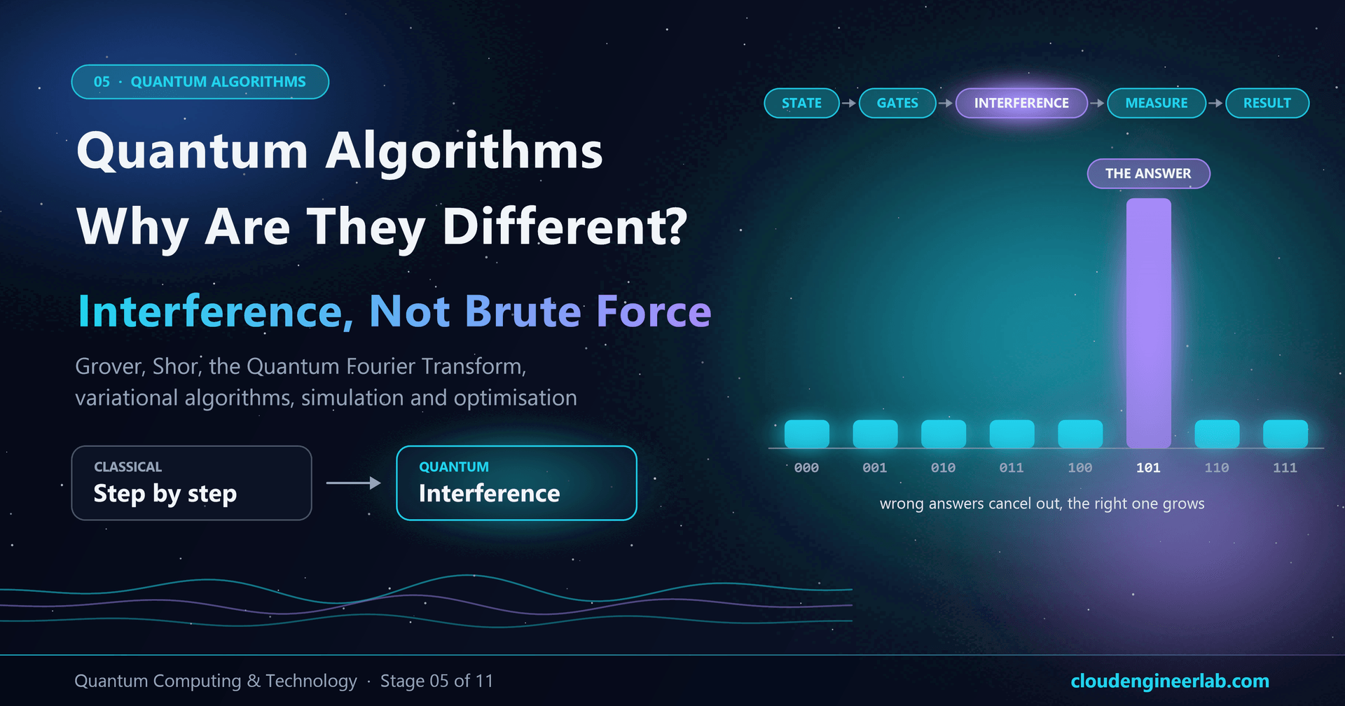
Quantum Algorithms: Why Are They Different?
How Grover, Shor, the Quantum Fourier Transform, variational algorithms, quantum simulation and optimisation work, and where quantum advantage really comes from.
Ask most people how a quantum computer would solve a problem and you'll hear something like: "It tries every possible answer at the same time." It's an appealing idea, and it's wrong in a way that matters. If that were how quantum computers worked, they would speed up everything. They don't. They speed up a short, specific list of problems, sometimes dramatically, and offer nothing at all for the rest.
To understand why, you need to understand what makes a quantum algorithm different from a classical one. Not with equations, but by looking at what each kind of algorithm actually does, step by step. That's where this post starts. Then it walks through the algorithms everyone talks about (Grover's search, the Quantum Fourier Transform, Shor's factoring, quantum simulation, variational algorithms and optimisation) and ends with the question that matters most: where could quantum advantage actually come from?
Stage 05 of the learning path
This is the opening post of stage 05, Quantum Algorithms, in the Quantum Computing & Technology learning path. It uses the gates from Quantum Gates Explained and the idea of interference from Superposition, Entanglement and Measurement Explained. Every circuit and result below was checked on Qiskit 2.5.2.
Two Different Ways to Compute
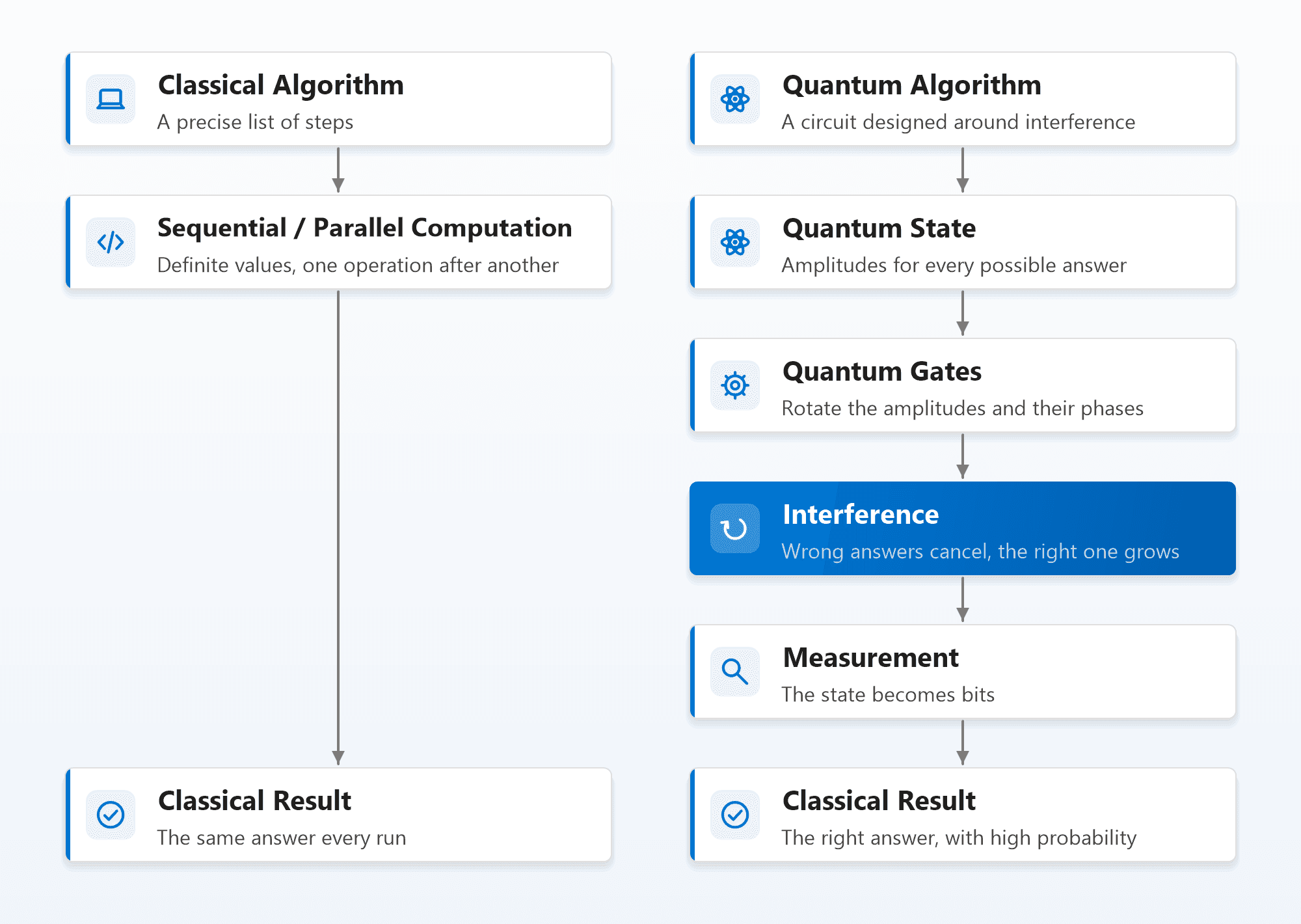
The classical path
A classical algorithm is a precise list of steps that act on definite values. Compare these two numbers, add those, store the result, move on. Speed comes from two places: making each step fast, and doing as few steps as possible. Parallel computers (multi-core CPUs, GPUs) run many steps at once, but each step still works on ordinary, definite values. Run the same program on the same input and you get the same result, every time.
The quantum path
A quantum algorithm takes a detour through four stages:
- Quantum state. The qubits are prepared, usually with Hadamard gates, into a superposition that has an amplitude for every possible answer at once.
- Quantum gates. A carefully designed sequence of gates rotates those amplitudes and, crucially, changes their phases (their signs, in the simplest case).
- Interference. The gates are arranged so that the amplitudes of wrong answers cancel out, and the amplitude of the right answer builds up. This is the heart of every quantum algorithm.
- Measurement. The state collapses to one classical result. Because interference has made the right answer far more likely than the others, that's usually what you get.
The detour only pays off if the third step works. The superposition holds every answer, but measurement only gives you one, chosen at random. Without interference, a quantum computer is just an expensive random number generator. With it, the random result is very likely to be the right one.
The one idea to take away
A quantum algorithm doesn't win by checking every answer in parallel. It wins by choreographing interference so that wrong answers cancel and the right one survives measurement. That's only possible for problems with the right kind of structure, which is why the list of good quantum algorithms is short.
Grover's Algorithm: Search by Interference
Grover's algorithm (1996) is the clearest example of interference at work. The problem: you have a list of N items and a way to recognise the right one, but no way to know where it is. Classically, you have to check items one by one: on average N/2 checks. Grover's algorithm needs only about √N steps.
How it works, on four items
Here is Grover's search on 4 possible answers (two qubits), where the answer we want is 11:
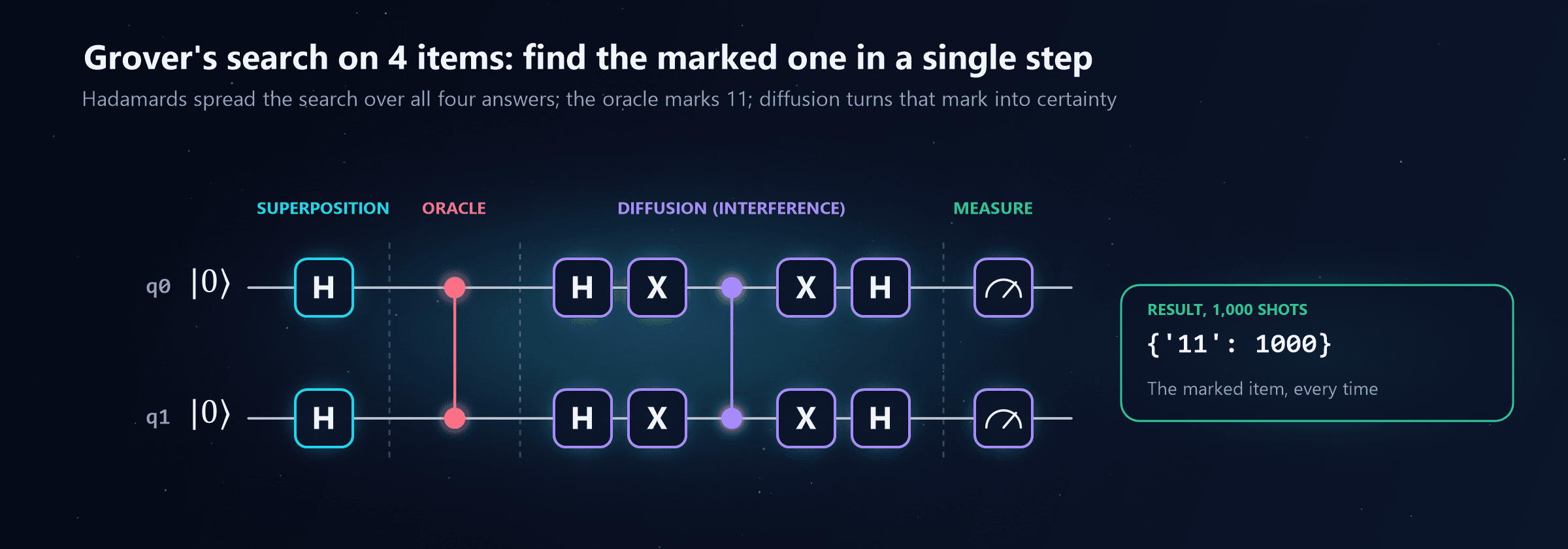
It has two repeating ingredients:
- The oracle recognises the answer. It doesn't reveal where the answer is; it just flips the sign of its amplitude, a phase flip that measurement can't see.
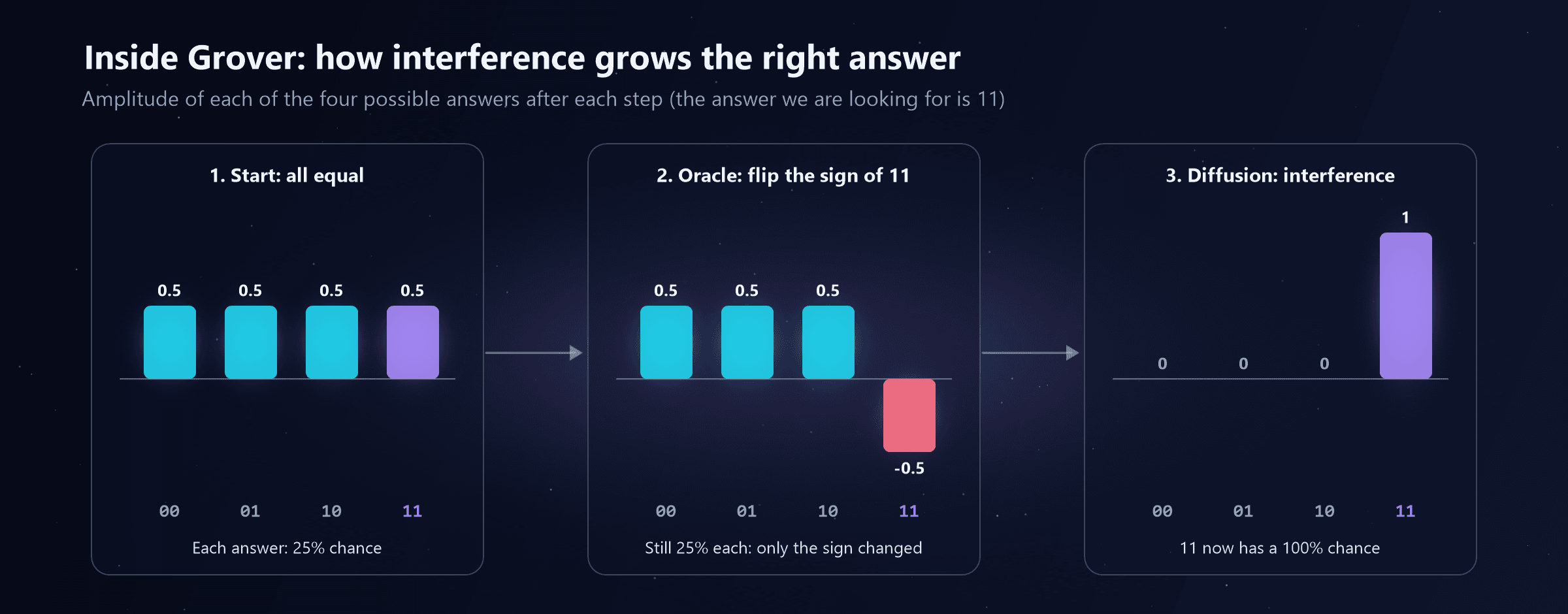
- The diffusion step performs interference. It reflects every amplitude around the average, which shrinks the unmarked answers and grows the one whose sign was flipped.
You can watch the amplitudes change:
And in code, the same circuit:
from qiskit import QuantumCircuit
from qiskit.primitives import StatevectorSampler

qc = QuantumCircuit(2, 2)
qc.h([0, 1])                     # superposition over 00, 01, 10, 11
qc.cz(0, 1)                      # oracle: flip the sign of 11
qc.h([0, 1]); qc.x([0, 1])       # diffusion: reflect about the average
qc.cz(0, 1)
qc.x([0, 1]); qc.h([0, 1])
qc.measure([0, 1], [0, 1])

print(StatevectorSampler().run([qc], shots=1000).result()[0].data.c.get_counts())
# {'11': 1000}
More steps are not always better
With more items, one round isn't enough, so the oracle and diffusion are repeated. But here's a surprise. Running Grover's search on 8 items (three qubits) in the test for this post gave:
| Rounds of oracle + diffusion | Chance of finding the marked item |
|---|---|
| 1 | 78.1% |
| 2 | 94.5% |
| 3 | 33.0% |
The third round made it worse. Interference keeps rotating the state, and if you go past the right point, you rotate away from the answer again. The ideal number of rounds is about π/4 × √N, and a Grover search has to stop there. It's a vivid reminder that quantum algorithms are precision choreography, not brute force.
How big is the speed-up?
| Items to search (N) | Classical checks (average) | Grover rounds |
|---|---|---|
| 4 | 2 | 1 |
| 1,000,000 | 500,000 | 785 |
| 1,000,000,000,000 | 500,000,000,000 | 785,398 |
That's a quadratic speed-up: the square root of the classical effort. It's real and proven, but it comes with two important caveats. First, you need an oracle that can recognise the answer, built from quantum gates. Second, each Grover round on real, error-corrected hardware is far slower than a classical check. Researchers have estimated that, once error-correction overheads are included, quadratic speed-ups may need very large problems before they beat a fast classical computer, and for some realistic problems they may never pay off.
The Quantum Fourier Transform: Finding Hidden Rhythm
The Quantum Fourier Transform (QFT) isn't a complete algorithm. It's a building block inside the most powerful ones, including Shor's.
What a Fourier transform does, without equations. Play a chord on a piano and a microphone records one messy, wiggly signal. A Fourier transform takes that signal apart and tells you which notes, at which frequencies, make it up. More generally, it finds repeating patterns: if something repeats every 4 steps, a Fourier transform reveals the 4. Classical computers use Fourier transforms everywhere, in audio and image compression, Wi-Fi, medical scanners and more.
What's different about the quantum version. The QFT performs the same transformation on the amplitudes of a quantum state. Here's the circuit for three qubits:
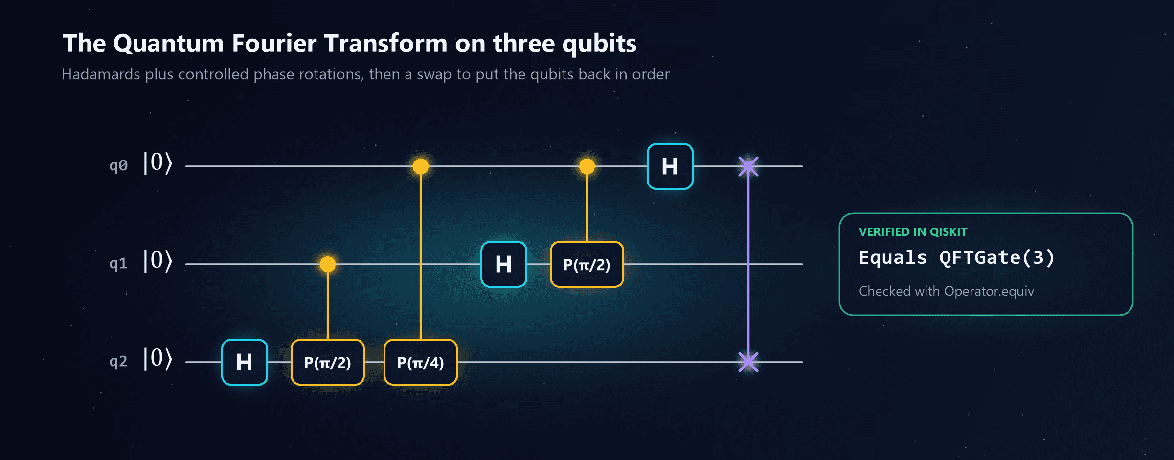
In Qiskit you'd normally use the built-in version:
from qiskit import QuantumCircuit
from qiskit.circuit.library import QFTGate

qc = QuantumCircuit(3)
qc.append(QFTGate(3), [0, 1, 2])   # the same transformation as the circuit above
Why it's powerful. On n qubits, the QFT transforms 2ⁿ amplitudes using only about n² gates. A classical fast Fourier transform on 2ⁿ numbers needs work proportional to 2ⁿ × n. For 50 qubits, that's the difference between a few thousand gates and around 50 quadrillion operations.
The catch. You can't read the 2ⁿ transformed amplitudes out; measurement gives you only n bits. So the QFT is only useful inside an algorithm that arranges for the one piece of information you need, such as the length of a repeating pattern, to come out when you measure. That's exactly what Shor's algorithm does.
Shor's Algorithm: Why Encryption Teams Care
Shor's algorithm (1994) is the reason governments and security teams pay attention to quantum computing. It finds the prime factors of large numbers, and with a related algorithm, solves the "discrete logarithm" problem. Those two problems are what keep RSA and elliptic-curve cryptography secure: the public-key encryption behind HTTPS, VPNs, code signing and the certificates in your PKI.
The clever reduction: factoring becomes rhythm-finding
Shor's insight was that factoring can be turned into finding a repeating pattern, the job the QFT is built for. Here's the idea with a number small enough to do by hand. To factor 15, pick a number, say 7, and look at the remainders when you divide its powers by 15:
| Power of 7 | Result | Remainder after dividing by 15 |
|---|---|---|
| 7¹ | 7 | 7 |
| 7² | 49 | 4 |
| 7³ | 343 | 13 |
| 7⁴ | 2,401 | 1 |
| 7⁵ | 16,807 | 7 (and the pattern repeats) |
The remainders repeat every 4 steps. That repeat length is called the period. Once you know it, a little classical arithmetic does the rest: take 7 to the power of half the period (7² = 49), then look at 49 − 1 = 48 and 49 + 1 = 50. The greatest common divisor of 48 and 15 is 3, and of 50 and 15 is 5. And 3 × 5 = 15. (This post's test script checked every one of those numbers.)
Where the quantum part comes in
For 15, you can spot the period by eye. For a 2048-bit RSA number, the pattern could be astronomically long, and no classical method can find it efficiently. Shor's algorithm uses a quantum computer for exactly that one step:
- Put a register of qubits into a superposition of every power.
- Compute the remainders for all of them at once, which entangles each power with its remainder.
- Apply the QFT, which makes the amplitudes interfere so that results related to the period reinforce each other and everything else cancels.
- Measure, and use classical arithmetic to read off the period.
Everything else, choosing the number, checking the answer and computing the factors, is classical.
How close is it?
Not close today, but closer than it used to look. Running Shor's algorithm on numbers that matter needs a large, fault-tolerant quantum computer, far beyond today's machines; the factoring demonstrations so far have only handled tiny numbers. But the estimates keep falling. In 2019 a well-known estimate for breaking 2048-bit RSA needed around 20 million noisy physical qubits; a 2025 update by the same researcher brought that below one million, running for under a week. That's still far beyond current hardware, but it's why organisations are being told to move to post-quantum cryptography now: encrypted data captured today could be decrypted once such a machine exists. Stages 08 and 09 of this path cover what to do about it.
Quantum Simulation: Using Nature to Model Nature
In 1981, physicist Richard Feynman made the observation that started the whole field: nature is quantum, so simulating it on classical computers is hopelessly hard, but a computer that is itself quantum could do it naturally.
Why classical computers struggle. Describing a molecule exactly requires keeping track of how all its electrons behave together. Each electron added roughly doubles the amount of information involved, so exact simulation quickly becomes impossible. Classical chemists use clever approximations, and they work remarkably well for many molecules, but they break down for exactly the ones that are most interesting: catalysts, complex magnetic materials, and materials where electrons interact strongly.
What a quantum computer does differently. It represents the molecule's electrons directly with qubits, and applies gates that mimic how the electrons interact over time (Hamiltonian simulation). Combined with an algorithm called quantum phase estimation, which uses the QFT, it can calculate quantities chemists care about, such as how much energy a reaction releases.
Why it's the most promising application. It has the strongest theoretical case for a large speed-up on problems people genuinely want solved:
- Chemistry: better catalysts for fertiliser production or carbon capture, and better understanding of how drugs bind.
- Materials: battery electrodes, solar materials, superconductors.
- Physics: the behaviour of exotic materials and particles.
Most of the high-value versions still need fault-tolerant machines, but simulation of simple physical models is already one of the main ways today's hardware is tested. Stage 07, Quantum Applications, looks at these use cases in detail.
Variational Quantum Algorithms: Teamwork With a Classical Computer
Algorithms like Shor's need thousands of perfect, error-corrected qubits. Variational quantum algorithms were designed for the noisy machines we actually have, by giving most of the work to a classical computer.
The idea is a loop:
It's similar in spirit to training a neural network: a model with adjustable parameters, a score, and an optimiser that nudges the parameters to improve the score. The quantum circuit is short, so it finishes before noise ruins it, and the classical computer does the heavy lifting. The rotation gates from the gates post are the adjustable knobs.
The two best-known examples:
- VQE (Variational Quantum Eigensolver) searches for the lowest energy of a molecule, a central quantity in chemistry.
- QAOA (Quantum Approximate Optimisation Algorithm) searches for good solutions to optimisation problems, such as dividing a network into two groups with as many connections between them as possible.
The honest picture. Variational algorithms run on today's hardware and are a valuable way to learn and benchmark, but there is no proof they beat the best classical methods, and they have practical problems. They need huge numbers of shots to estimate each score accurately. For larger circuits, the "landscape" the optimiser explores can become almost completely flat (a problem called barren plateaus), leaving the optimiser lost. They're best seen as an active research bet, not a solved route to advantage.
Optimisation Algorithms: Promising, Popular and Unproven
Optimisation (finding the best route, schedule, portfolio or configuration among a vast number of options) is where the business interest in quantum computing is highest. It's also where claims most need checking.
The main quantum approaches:
| Approach | How it works | Status |
|---|---|---|
| QAOA | Variational circuits that alternate between "score the options" and "mix the options" steps | Heavily studied on small problems; no demonstrated practical advantage |
| Quantum annealing | A special-purpose machine (such as D-Wave's) slowly relaxes a physical system into a low-energy state that encodes a good solution | Commercially available; advantage over classical methods remains debated |
| Grover-based search | Uses Grover-style amplification to search for better solutions | At most a quadratic speed-up, and needs fault-tolerant hardware |
The most important fact about optimisation. The hardest optimisation problems (known as NP-hard problems, which include many scheduling and routing problems) are not believed to be efficiently solvable by quantum computers either. Quantum computers are not expected to make them easy. At best, they might give a modest speed-up, or better approximate answers for particular kinds of problem. Meanwhile, classical optimisation software is extremely good and keeps improving, which raises the bar for any quantum method.
That doesn't make quantum optimisation pointless. It makes it an open question, and it means any claim of "quantum-optimised logistics" deserves a close look at what it was compared against.
Where Could Quantum Advantage Come From?
With all six in view, the pattern becomes clear. Quantum advantage isn't spread evenly across computing. It comes from a few specific sources:
| Algorithm | Problem it solves | Best classical approach | Expected quantum speed-up | Needs fault tolerance? |
|---|---|---|---|---|
| Shor | Factoring and discrete logarithms (breaks RSA and ECC) | Grows almost exponentially with key size | Super-polynomial: enormous | Yes |
| Quantum simulation | Molecules, materials, physics | Cost explodes with system size for hard cases | Exponential for some problems | Mostly yes |
| QFT | A building block for period-finding and phase estimation | Fast Fourier transform | Exponential inside other algorithms; not on its own | Yes, inside larger algorithms |
| Grover | Unstructured search | Check items one by one | Quadratic | Yes, for useful sizes |
| Amplitude estimation | Monte Carlo-style estimation (risk, pricing) | Repeated random sampling | Quadratic | Yes |
| Variational (VQE, QAOA) | Chemistry, optimisation | Strong classical heuristics | Unproven | Designed not to need it |
| Optimisation in general | Routing, scheduling, portfolios | Excellent heuristics | At most modest; unproven in practice | Varies |
Three requirements show up again and again:
- Hidden structure. The problem must contain something interference can exploit: a repeating pattern (Shor), the structure of quantum physics itself (simulation), or at least a way to recognise the answer (Grover). Problems without such structure get no speed-up.
- Small input, hard computation. Quantum computers can't load large datasets quickly, and they can only output a few bits per run. They suit problems where the question is short (one number to factor, one molecule to model) but the computation is enormous.
- A result you can use. Since you can't read out the whole quantum state, the algorithm has to concentrate the answer into something measurement can reveal.
And the thing quantum advantage does not come from: "trying every answer in parallel". Every quantum algorithm that works does so because of interference, not because of parallelism.
Quantum advantage is a moving target
Claims of quantum advantage have a habit of being challenged, which is a healthy part of science:
- In 2019, Google reported that its Sycamore processor completed a sampling task in minutes that would take a supercomputer thousands of years. Later, improved classical methods brought that classical estimate down dramatically.
- In 2023, IBM published an experiment showing useful results on a 127-qubit processor beyond simple classical simulation. Within weeks, several groups showed that clever classical methods could reproduce it.
- In 2024, Google's Willow chip ran a random sampling benchmark in under five minutes that it estimated would take the fastest supercomputers vastly longer than the age of the universe. In 2025, Google reported a "verifiable" advantage on a physics simulation task; as with every such claim, the community continues to test it.
- Some proposed quantum algorithms, such as one for recommendation systems, were later "dequantised": researchers found classical algorithms that perform almost as well.
The lesson isn't that quantum advantage is fake. It's that advantage is defined relative to the best classical method, which keeps improving. The most convincing cases are problems where there are strong theoretical reasons to believe classical computers can't catch up, which is exactly why Shor's algorithm and quantum simulation dominate serious roadmaps.
How to Read a Quantum Algorithm Claim
1. What was it compared against?
2. Is the speed-up proven or hoped for?
3. Does the problem have exploitable structure?
4. What about input and output?
5. Does it need fault tolerance?
Quick Recap
- Classical algorithms follow steps on definite values; quantum algorithms detour through a quantum state and use interference before measuring.
- Interference, not parallelism, is the source of every real quantum speed-up.
- Grover searches with a proven quadratic speed-up, and over-running it makes the answer less likely.
- The QFT finds repeating patterns in amplitudes with very few gates, but only works inside larger algorithms.
- Shor turns factoring into period-finding, threatening RSA and ECC once fault-tolerant machines exist.
- Quantum simulation is the most promising application, because nature itself is quantum.
- Variational algorithms share work with classical computers to run on noisy hardware, but have no proven advantage.
- Optimisation is popular and important, but NP-hard problems are not expected to become easy, and advantage is unproven.
- Advantage is relative to the best classical method, and that target keeps moving.
What's Next on the Learning Path
Stage 06, Quantum + AI, starts with Why Is Quantum Computing Accelerating Now? and then looks at the two technologies everyone mentions together: what quantum computers might, and might not, do for machine learning, and how AI is already helping to build better quantum computers. The full 11-stage path is listed at the end of the beginner's guide.

Written by
Chetan Yamger
Cloud Engineer · AI Automation Architect · Modern Workplace Consultant
Cloud Engineer, AI Automation Architect, and Modern Workplace Consultant based in Amsterdam, Netherlands. Specializing in scalable, secure enterprise solutions with Microsoft Azure, Intune, PowerShell, and AI-driven automation using ChatGPT, Gemini, and modern LLM technologies.
Stay in the loop.
New articles, straight to you.
Deep-dive technical articles on Intune, PowerShell, and AI — no noise, no spam.
Discussion
Share your thoughts — your email stays private
Leave a comment