
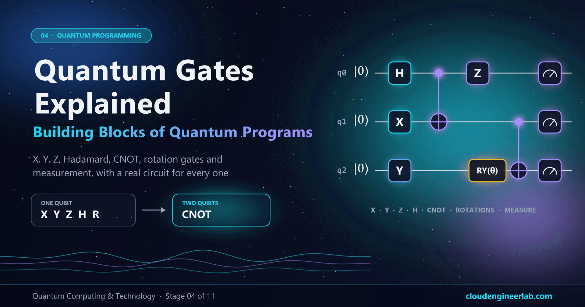
Quantum Gates Explained: The Building Blocks of Quantum Programs
X, Y, Z, Hadamard, CNOT, rotation gates and measurement explained with a real circuit diagram, Qiskit code and tested results for every gate.
In your first quantum program you used two instructions, a Hadamard gate and a measurement, and watched a qubit produce random 0s and 1s. Real quantum programs use the same idea with a slightly bigger toolbox.
That toolbox is surprisingly small. A handful of quantum gates (X, Y, Z, Hadamard, CNOT and rotations), plus measurement, is enough to build every quantum algorithm ever written. This post introduces each one, the way a programmer meets a new instruction: what it does, how to write it, what the circuit looks like, and what you get when you run it.
Stage 04 of the learning path
This post is part of stage 04, Quantum Programming, in the Quantum Computing & Technology learning path. It follows Your First Quantum Program, so you already have Qiskit installed. Every circuit below was run on Qiskit 2.5.2 with 1,000 shots, and each diagram shows the real result. Paste the code and you'll see the same pattern; probabilistic counts will vary slightly from run to run.
How the Pieces Fit Together
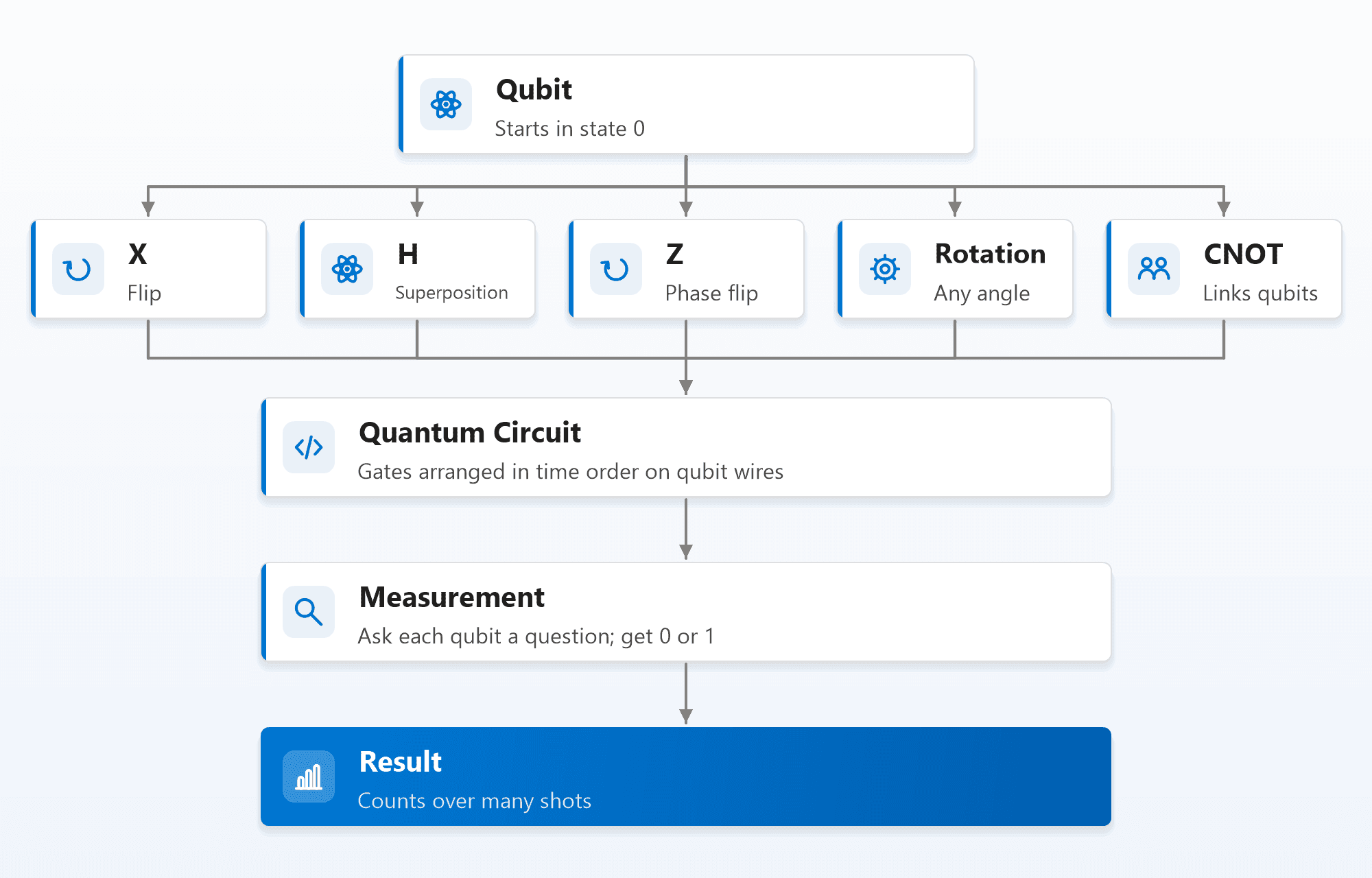
Three ideas will make every gate in this post easier to understand:
- A gate is a rotation. Picture a qubit's state as a point on a sphere, with 0 at the north pole and 1 at the south pole (the Bloch sphere). Every single-qubit gate turns that point around some axis. Only the latitude (how far north or south) decides the chances of measuring 0 or 1. The longitude is the phase, which you can't see directly but which decides how qubits interfere later.
- Gates are reversible. Every quantum gate can be undone by another gate. Nothing is thrown away until you measure.
- Circuits read left to right. Each horizontal line is one qubit, and time flows from left to right, exactly like the diagrams below.
The X Gate: a Quantum NOT
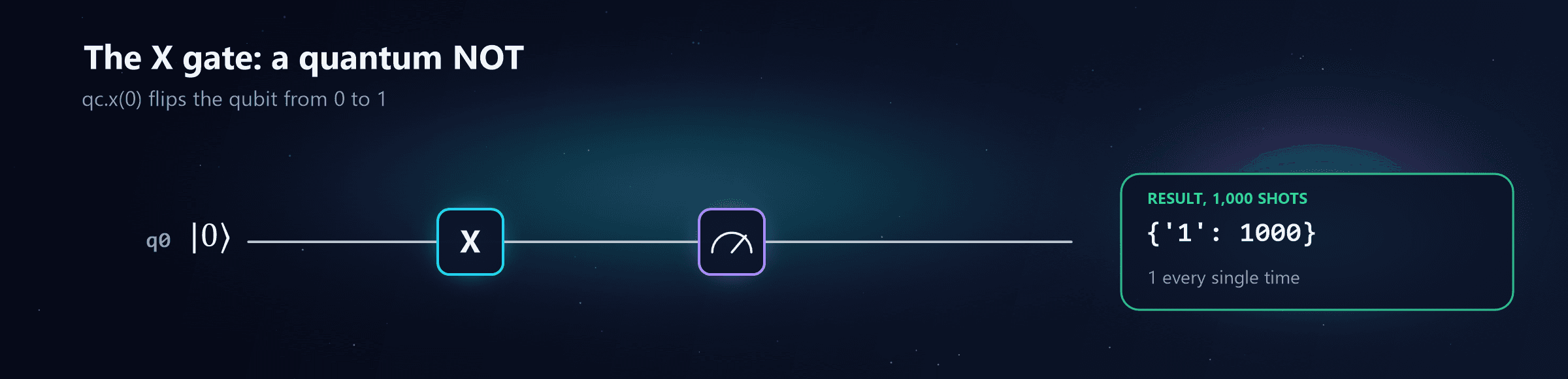
from qiskit import QuantumCircuit
from qiskit.primitives import StatevectorSampler

qc = QuantumCircuit(1, 1)
qc.x(0)            # X gate on qubit 0
qc.measure(0, 0)

print(StatevectorSampler().run([qc], shots=1000).result()[0].data.c.get_counts())
# {'1': 1000}
What it does. X swaps 0 and 1: a qubit in 0 becomes 1, a qubit in 1 becomes 0. It's the quantum version of the classical NOT gate. On the Bloch sphere, it's a half-turn around the X axis, which carries the north pole to the south pole.
Where you'll use it. To set a qubit to 1 at the start of a circuit, and inside larger gates (CNOT is "X, but only if another qubit is 1").
One difference from NOT. If the qubit is in a superposition, X swaps the two amplitudes instead of flipping a single value, so it acts on both possibilities at once.
The Y Gate: a Flip With a Twist
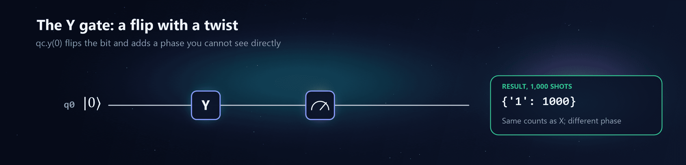
qc = QuantumCircuit(1, 1)
qc.y(0)            # Y gate on qubit 0
qc.measure(0, 0)
# {'1': 1000}
What it does. Y is a half-turn around the Y axis. Like X, it swaps 0 and 1, so measuring straight afterwards gives the same result as X. But it also adds a phase: if you inspect the state on a simulator, Y turns 0 into a 1 with an amplitude of i (the imaginary unit) rather than plain 1.
Why it matters. On its own, you'd never notice the difference. In a longer circuit, where that phase can interfere with other paths, X and Y behave differently. Y is used less often than X or Z in everyday programs, but it completes the set: X, Y and Z are the three half-turns around the sphere's three axes.
The Z Gate: Invisible Until It Interferes
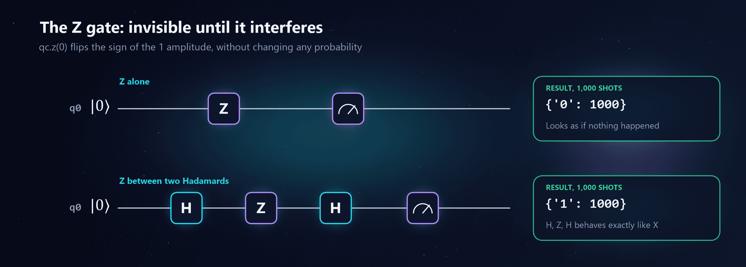
qc = QuantumCircuit(1, 1)
qc.z(0)
qc.measure(0, 0)
# {'0': 1000}        <- Z alone: no visible change

qc = QuantumCircuit(1, 1)
qc.h(0)
qc.z(0)
qc.h(0)
qc.measure(0, 0)
# {'1': 1000}        <- H, Z, H: the phase flip becomes a bit flip
What it does. Z leaves 0 alone and flips the sign of the 1 amplitude. On the Bloch sphere, it's a half-turn around the vertical Z axis. Because that turn doesn't change the latitude, the probabilities of 0 and 1 never change: measuring straight after a Z shows nothing at all.
Why it matters. Z changes the phase, and phase is what decides interference. The second circuit shows this. Hadamard moves the qubit onto the equator, Z swings it to the opposite side, and the second Hadamard turns that sign difference into a definite 1. In fact, H followed by Z followed by H is exactly the same operation as X, a neat identity worth remembering.
Z is everywhere in real algorithms: it's how a quantum algorithm "marks" an answer without measuring it, so that interference can amplify it later.
The Hadamard Gate: Into Superposition and Back
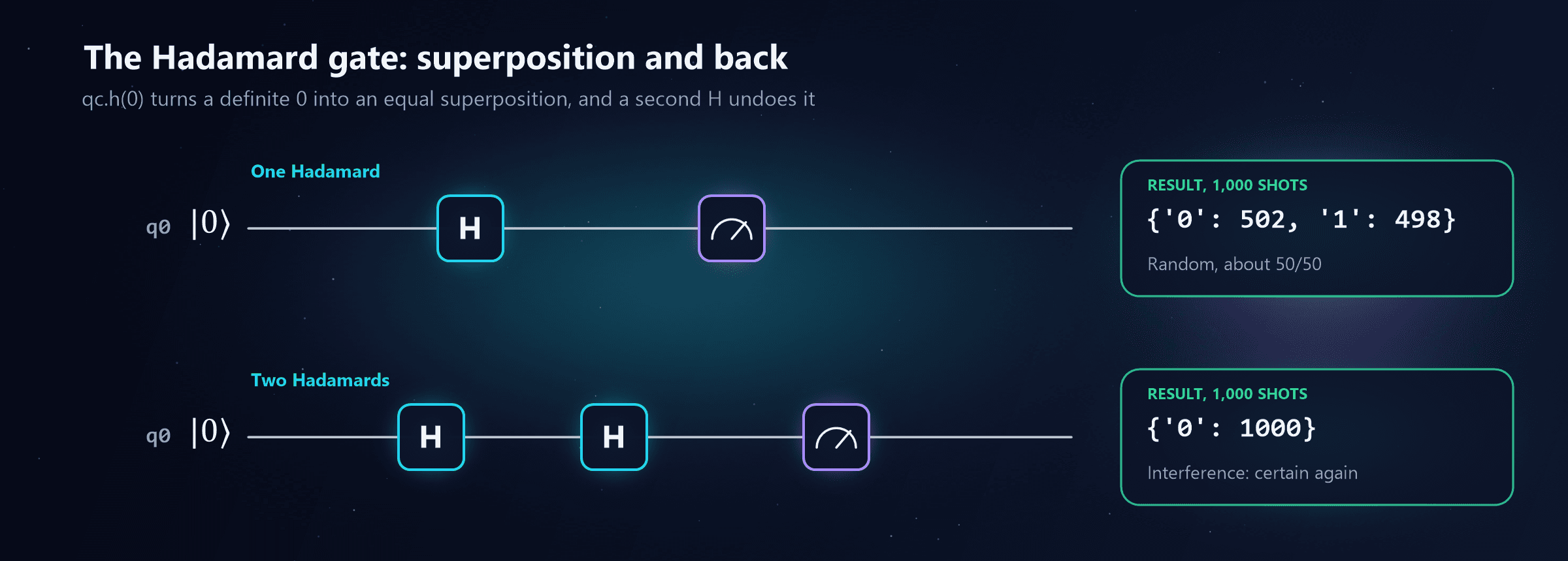
qc = QuantumCircuit(1, 1)
qc.h(0)
qc.measure(0, 0)
# {'0': 502, '1': 498}   <- one H: equal superposition

qc = QuantumCircuit(1, 1)
qc.h(0)
qc.h(0)
qc.measure(0, 0)
# {'0': 1000}            <- two H: interference, certain again
What it does. The Hadamard (H) turns 0 into an equal superposition called "plus", and 1 into an equal superposition called "minus" (same probabilities, opposite sign). It is its own inverse: applying it twice returns the original state.
Why it matters. H is the most important single gate in quantum computing. Almost every algorithm starts by applying H to many qubits at once, to create a superposition across all their combinations, and many end with H again to turn phase differences into measurable results. It's also the gate that switches between the "0 or 1" view of a qubit and the "plus or minus" view, which you'll see again in the measurement section.
CNOT: the Gate That Links Two Qubits
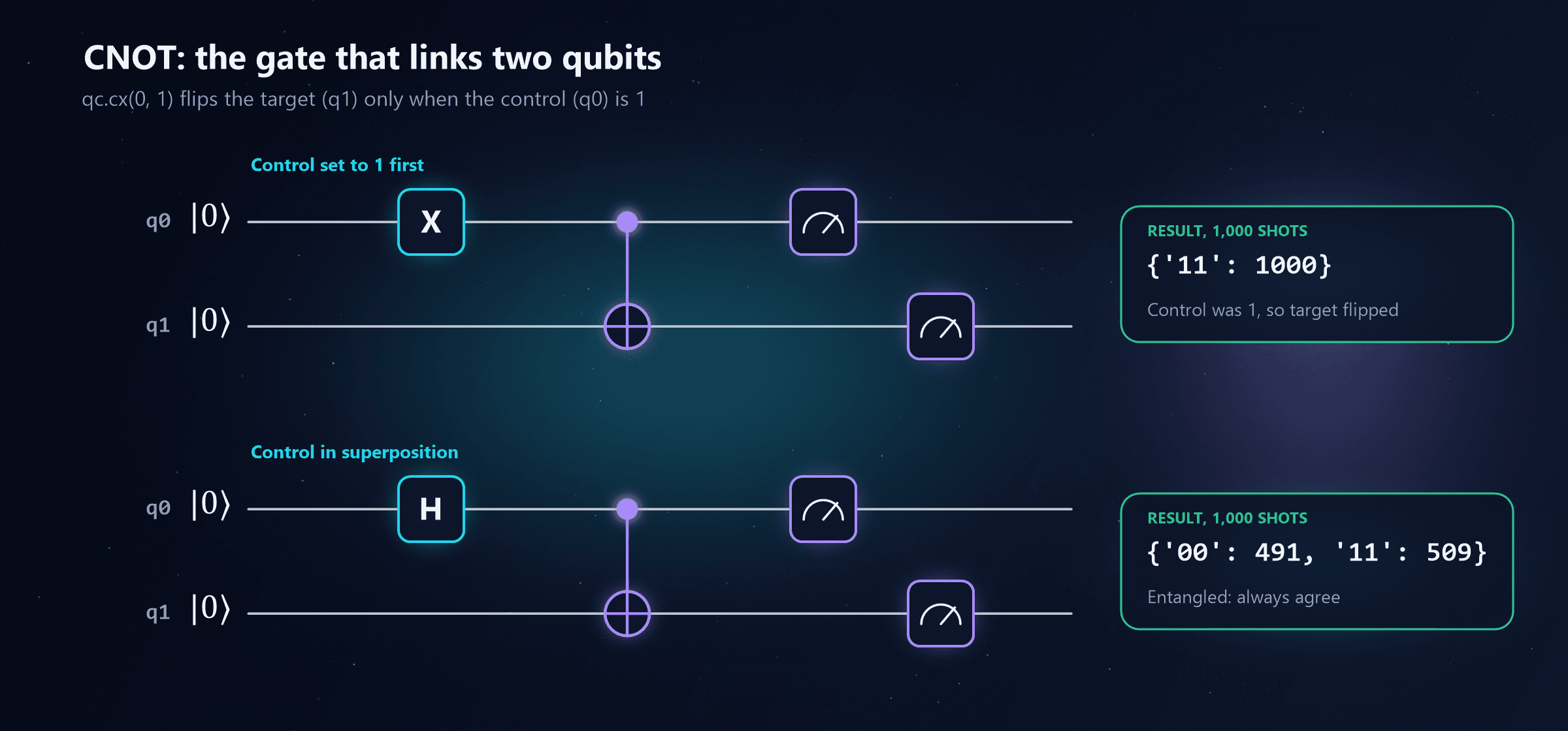
qc = QuantumCircuit(2, 2)
qc.x(0)                 # set the control to 1
qc.cx(0, 1)             # CNOT: control q0, target q1
qc.measure([0, 1], [0, 1])
# {'11': 1000}

qc = QuantumCircuit(2, 2)
qc.h(0)                 # control in superposition
qc.cx(0, 1)
qc.measure([0, 1], [0, 1])
# {'00': 491, '11': 509}  <- the Bell state: entangled
What it does. CNOT (controlled-NOT, written cx in Qiskit) acts on two qubits. If the control qubit is 1, it flips the target qubit. If the control is 0, it does nothing. In circuit diagrams, the control is a filled dot and the target is a circle with a cross through it, joined by a vertical line.
| Control (q0) | Target (q1) before | Target (q1) after |
|---|---|---|
| 0 | 0 | 0 |
| 0 | 1 | 1 |
| 1 | 0 | 1 |
| 1 | 1 | 0 |
Why it matters. With definite inputs, CNOT is just a reversible classical gate. But when the control is in a superposition, as in the second circuit, the "flip or don't flip" decision happens in superposition too, and the two qubits end up in one shared, entangled state. CNOT plus single-qubit gates is all you need to create entanglement, which is why it's the standard two-qubit gate in almost every quantum computer.
Watch the bit order in Qiskit
Qiskit writes results with qubit 0 on the right. So the string '10' means q1 is 1 and q0 is 0. When this post's test ran the CNOT truth table, the input "control 0, target 1" came back as '10', not '01'. It's the most common source of confusion in multi-qubit results. With symmetric results like '00' and '11' it doesn't matter, but with anything else it does.
Rotation Gates: Dial In Any Probability
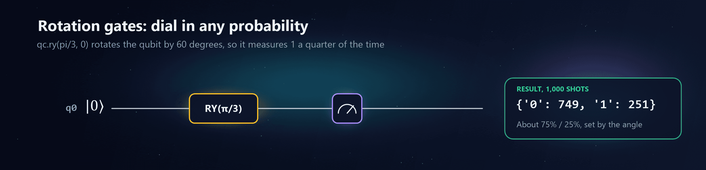
from math import pi

qc = QuantumCircuit(1, 1)
qc.ry(pi / 3, 0)        # rotate by 60 degrees around the Y axis
qc.measure(0, 0)
# {'0': 749, '1': 251}
What they do. X, Y and Z are fixed half-turns. Rotation gates let you choose the angle: rx(θ), ry(θ) and rz(θ) turn the qubit by any angle θ around the X, Y or Z axis. The angle is written in radians, so π is a half-turn (180°) and π/2 is a quarter-turn (90°).
For ry, the chance of measuring 1 is set directly by the angle:
Angle θ in ry(θ) | In degrees | Chance of 0 | Chance of 1 |
|---|---|---|---|
| 0 | 0° | 100% | 0% |
| π/3 | 60° | 75% | 25% |
| π/2 | 90° | 50% | 50% (same as H, for these probabilities) |
| π | 180° | 0% | 100% (same as X, up to a phase) |
Related phase gates. rz changes only the phase. Two fixed versions have their own names: S is a quarter-turn around Z (two S gates make a Z), and T is an eighth-turn (two T gates make an S). They look minor, but T has a special role: it's the gate that's hardest to perform on error-corrected hardware, as the error correction deep dive explains.
Why they matter. Rotations are how quantum programs get tuneable knobs. Many practical algorithms, especially in chemistry and machine learning, are built from rotation gates whose angles are adjusted by a classical optimiser, run after run, until the circuit gives the best answer. They're also what real hardware uses internally: on IBM's chips, for example, an rz rotation costs no time at all (it's done in software), which is why compiled circuits are full of them.
Measurement: Not a Gate, but the Step That Gives You an Answer
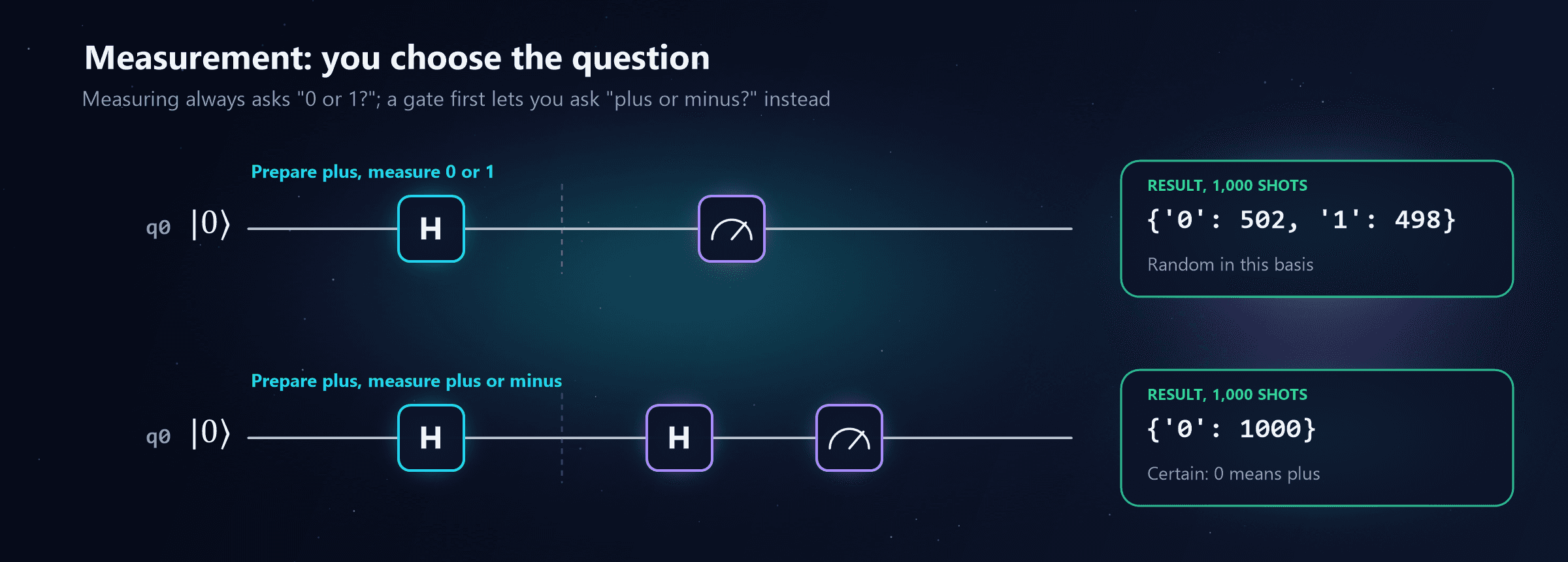
qc = QuantumCircuit(1, 1)
qc.h(0)              # prepare the "plus" state
qc.h(0)              # change basis: now "0" means plus and "1" means minus
qc.measure(0, 0)
# {'0': 1000}
What it does. Measurement asks each qubit "0 or 1?" and returns one classical bit, chosen at random with probabilities set by the state. Afterwards, the superposition is gone.
Why it isn't a gate. Every gate is reversible; measurement is not. You can't undo it, and you can't recover the amplitudes that produced the result. That's why circuit diagrams draw it differently, as a meter rather than a box with a letter.
You choose the question. Hardware can only measure "0 or 1?" directly. To ask a different question, you rotate the qubit first. Applying H before measuring turns the question into "plus or minus?". In the second circuit, the qubit was prepared in "plus", so that question gets a certain answer, while the "0 or 1?" question in the first circuit gets a random one. Choosing which question to ask is part of designing an algorithm, and it's the heart of protocols like quantum key distribution.
Superposition, Entanglement and Measurement Explained covers the five rules of measurement in detail.
Putting It Together: a Three-Qubit Circuit
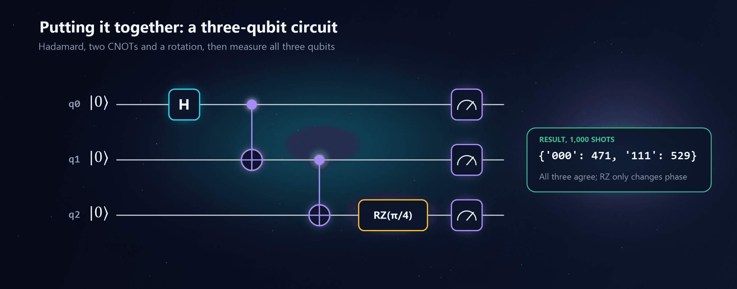
from math import pi
from qiskit import QuantumCircuit
from qiskit.primitives import StatevectorSampler

qc = QuantumCircuit(3, 3)
qc.h(0)
qc.cx(0, 1)
qc.cx(1, 2)
qc.rz(pi / 4, 2)
qc.measure([0, 1, 2], [0, 1, 2])

print(qc)
print(StatevectorSampler().run([qc], shots=1000).result()[0].data.c.get_counts())
# {'000': 471, '111': 529}
Read it left to right:
- H puts q0 into a superposition.
- CNOT from q0 to q1 entangles them: they now always agree.
- CNOT from q1 to q2 extends that agreement to the third qubit. All three are now in one shared state, known as a GHZ state: all 0 or all 1.
- RZ rotates the phase of q2. It doesn't change the counts, because measuring "0 or 1?" can't see phase. In a longer algorithm, that phase could be turned into a visible difference by later gates, exactly as Z was in the H-Z-H circuit.
- Measurement gives 000 or 111, about half the time each.
Try changing it: remove the second CNOT and you'll see q2 stay at 0, or replace rz with ry and the clean 000/111 pattern breaks apart.
Quantum Gates Cheat Sheet
| Gate | Qiskit | Effect on 0 | Effect on 1 | On the Bloch sphere | Classical cousin |
|---|---|---|---|---|---|
| X | qc.x(q) | Becomes 1 | Becomes 0 | Half-turn around X | NOT |
| Y | qc.y(q) | Becomes 1 (with phase) | Becomes 0 (with phase) | Half-turn around Y | NOT, plus a phase |
| Z | qc.z(q) | Unchanged | Sign flipped | Half-turn around Z | None |
| H | qc.h(q) | Becomes plus (50/50) | Becomes minus (50/50) | Swaps the poles and the equator's plus and minus points | None |
| S, T | qc.s(q), qc.t(q) | Unchanged | Phase shifted | Quarter-turn and eighth-turn around Z | None |
| RX, RY, RZ | qc.rx(θ, q) and so on | Rotated by θ | Rotated by θ | Turn by any angle around X, Y or Z | None |
| CNOT | qc.cx(c, t) | Control 0: no change | Control 1: target flips | Two-qubit; creates entanglement | XOR |
| CZ | qc.cz(a, b) | No change unless both are 1 | Both 1: sign flipped | Two-qubit, symmetric | None |
| SWAP | qc.swap(a, b) | The two qubits exchange states | The two qubits exchange states | Built from three CNOTs | Swap |
| Toffoli | qc.ccx(a, b, t) | No change unless both controls are 1 | Both controls 1: target flips | Three-qubit | AND (reversible) |
| Measure | qc.measure(q, c) | Returns 0 | Returns 1 | Ends the superposition | Reading a bit |
For the curious: the matrices
Every gate can also be written as a small grid of numbers (a matrix) that transforms the two amplitudes. You never need these to write programs, but they're how gates are described in textbooks, so here are the four you'll meet most often.
X = [ 0  1 ]    Y = [ 0  -i ]    Z = [ 1   0 ]    H = 1/√2 × [ 1   1 ]
    [ 1  0 ]        [ i   0 ]        [ 0  -1 ]               [ 1  -1 ]
How Few Gates Do You Really Need?
Surprisingly few. Just as every classical program can be built from NAND gates alone, every quantum program can be built from a small universal gate set. One common choice is H, S, T and CNOT; another is rotation gates plus CNOT. Any other gate, however complicated, can be built from (or approximated by) a sequence of these.
That's why real quantum computers support only a few native gates and translate everything else. When you send a circuit to IBM hardware, the compiler rewrites your H into a combination of rz and sx gates, and your CNOT into the chip's own two-qubit gate plus rotations. You saw this happen in the first program's real-hardware step, and How Does a Quantum Computer Actually Work? shows how each native gate becomes a microwave pulse.
Quick Recap
- X flips 0 and 1, the quantum NOT.
- Y flips 0 and 1 and adds a phase.
- Z flips the phase of 1; invisible on its own, decisive in interference (H, Z, H equals X).
- H creates an equal superposition, and undoes it when applied twice.
- CNOT flips a target when the control is 1, and creates entanglement when the control is in superposition.
- Rotations turn a qubit by any angle, giving tuneable probabilities and phases; S and T are fixed phase rotations.
- Measurement isn't reversible; it asks "0 or 1?", and a gate beforehand chooses a different question.
- A small universal set of gates builds every quantum program, and real hardware compiles everything into its own native gates.
What's Next on the Learning Path
With the gates in hand, the next step is to combine them into something useful. Stage 05, Quantum Algorithms: Why Are They Different?, shows how gates like these are arranged so that interference makes the right answer come out, starting with the simplest algorithms that genuinely beat any classical approach. The full 11-stage path is listed at the end of the beginner's guide.

Written by
Chetan Yamger
Cloud Engineer · AI Automation Architect · Modern Workplace Consultant
Cloud Engineer, AI Automation Architect, and Modern Workplace Consultant based in Amsterdam, Netherlands. Specializing in scalable, secure enterprise solutions with Microsoft Azure, Intune, PowerShell, and AI-driven automation using ChatGPT, Gemini, and modern LLM technologies.
Stay in the loop.
New articles, straight to you.
Deep-dive technical articles on Intune, PowerShell, and AI — no noise, no spam.
Discussion
Share your thoughts — your email stays private
Leave a comment